HERMES
A differentiable pipeline for finding and vetting transiting exoplanets in Kepler photometry - and, because the whole thing is differentiable, an instrument for measuring what it actually does. Most of what I predicted about it turned out to be wrong.
- Vetter test ROC-AUC (Kepler photometry, 3,250 TCEs)
- 0.979
- Signal lost between duration templates in the search
- 9.4 pts
- Cost of locating the detection boundary, gradients vs bisection
- 4.1× fewer
- Predictability of the "physics-informed" feature from its neighbours
- R2 = 1.000000
- Effect of that feature on the trained classifier
- none measurable
Summary
I built a transit-detection pipeline in JAX: a matched-filter periodogram whose template is a limb-darkened transit, a differentiable Mandel-Agol fit that refines each candidate, and a dual-view CNN plus transformer that classifies it as a planet or a false positive. None of those components is new. What is unusual is that the search, the physical forward model and the classifier all live in one differentiable program, and that turns out to be useful for something other than training: the pipeline can measure itself.
I used that to ask three questions. Where does the search stop finding planets, and can gradients map that boundary more cheaply than brute force? Does the “physics-informed” feature the project was built around carry any information? And does any of it change what the classifier can do?
The answers, in order: the boundary can be traced about four times more cheaply, and doing so exposed two real defects in my own search. The physics feature, as I had implemented it, was an exact algebraic function of the features beside it
- it carried nothing. Fixing that made it genuinely informative in isolation, and still changed the classifier by an amount indistinguishable from zero.
Why machine learning at all
This is the first question anyone should ask, and it took me a while to answer it properly.
The forward problem is solved. Mandel & Agol (2002) give an exact, closed-form expression for the flux blocked when an opaque planet crosses a limb-darkened star. Given the orbital parameters, the light curve is a formula. The inverse problem is close to solved too: Seager & Mallén-Ornelas (2003) show that the four observables of a transit determine the system’s geometry analytically, and where that is not enough the field uses MCMC, which is well-understood and gives calibrated uncertainties. Neither is a learning problem.
What has no closed form is a false positive. A background eclipsing binary, diluted by an unrelated star inside a four-arcsecond Kepler pixel, with detector artefacts and starspot modulation at a near-harmonic period - there is no generative model for that. Deciding whether a periodic dip is a planet or one of those is the part that is genuinely a classification problem, and it is why AstroNet and its successors exist.
So the learned component here has one job, and it sits at the end of a classical pipeline. It never sees a raw light curve. It sees a phase-folded, depth-normalised summary of one, after the physics has already found and fitted the candidate.
Measuring the search instead of just running it
Whether a search finds an injected planet is one bit, and it costs a full periodogram to learn. I replaced the bit with a signed number:
margin(θ) = power at the injected period - strongest power anywhere unrelated to it
The search recovers the planet exactly when this is positive, so the detection boundary is where it crosses zero. Because the chain from transit parameters through phase binning to the matched filter is all JAX, the margin has a gradient with respect to the planet’s shape at fixed period.
Two checks that it is right. Against finite differences it agrees to a relative error of 3×10⁻⁶. And matched-filter power goes as depth2, which is the fourth power of the planet-to-star radius ratio, so d(margin)/d(log k) should be exactly four times the signal power. Measured: 4.005. That second check exercises the transit model, the binning and the correlation together, which is a stronger statement than “the gradient is finite”.
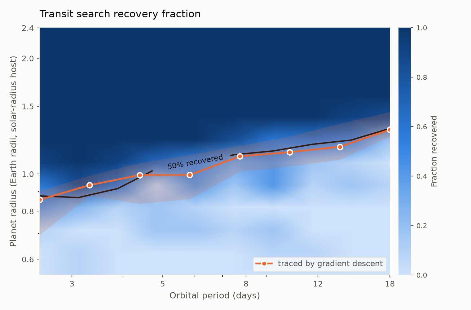
The two curves agree to a median of 1.4%. Bisection needs 14 periodogram evaluations per boundary point; Newton on the gradient needs a median of 4. That is 4.1× fewer searches and 2.2× faster in wall-clock - reverse-mode differentiation is not free, and wall clock is the honest number of the two. On the same noise realisation the two methods agree on the root to 0.07%.
This matters because detection efficiency is not a curiosity. Every occurrence-rate estimate, including every published figure for how common Earth-sized planets are, divides observed counts by it, and it is normally measured by injecting millions of synthetic transits.
This technique is not new, and I did not know that when I started. The gravitational-wave community has had a complete formalism for it since the 1990s - minimal match and fitting factor (Owen 1996; Owen & Sathyaprakash 1999), with template spacing derived from a metric built out of second derivatives of the match. What I call mismatch is their fitting factor. Applying it to transit search through automatic differentiation is the only uncommon part, and that is a matter of tooling rather than of insight.
What the search actually does
With the instrument working, I pointed it at my own search. I expected grazing transits to be its blind spot: the templates are all built at zero impact parameter, so a V-shaped grazing transit should be badly mismatched to a U-shaped template.
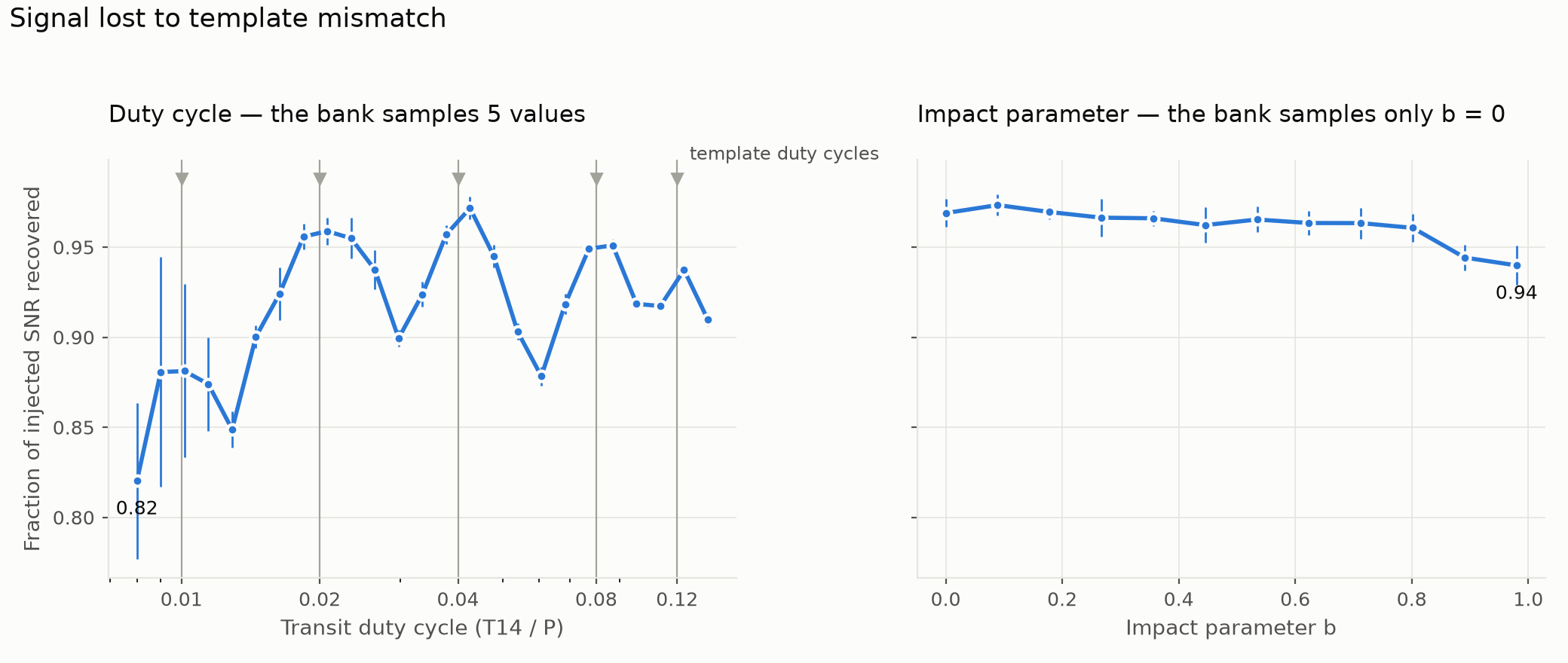
That was wrong. Across impact parameters from 0 to 0.98 the filter loses 2.9 points of signal-to-noise, most of it above b = 0.89. Grazing transits are hard to find because they are shallow - the injected signal drops from 178 to 54 - not because the templates mismatch them. A matched filter is more forgiving of shape than I assumed.
The duty cycle is where the loss is. The bank samples five discrete values, and a transit landing midway between two of them recovers 0.878 of its signal against 0.972 for one landing on a template: 9.4 points, about three times the cost of ignoring impact parameter entirely. The practical consequence is the opposite of my instinct - densify the duration grid, do not build V-shaped templates.
The scan also exposed a defect I would not have found by reading the code. Below
a duty cycle of about 0.012 the loss grew sharply and the scatter across noise
realisations exploded. That is not template mismatch. The period grid’s spacing
is derived from a min_duration_fraction parameter that defaulted to 0.05,
while the template bank searched duty cycles down to 0.01 - so short transits
were being searched on a grid too coarse to resolve them. Refining the grid
fourfold recovers 8.9 points at a duty cycle of 0.008 and changes nothing at
0.061, which separates the two failures cleanly: below 0.012 the grid binds,
between templates the bank binds, and refining the grid cannot help with the
second.
It matters most where it hurts most. Duty cycle falls with period - 0.016 at 10 days, 0.006 at 50, 0.0015 at a year - so long-period planets sit below the shortest template and on the undersampled part of the grid.
The physics feature that carried no information
The project’s distinguishing claim was a stellar-density consistency term. For a circular orbit, the transit’s geometry implies a stellar density; comparing it with the star’s catalogued density gives log(ρcirc / ρstar), which is near zero for a planet and large for a blended eclipsing binary. This is an old and genuinely good diagnostic (Seager & Mallén-Ornelas 2003; Kipping 2014). I used it as both an input feature and a training loss.
It carried no information whatsoever.
The scaled semi-major axis was computed by inverting the catalogued transit duration. Writing out the substitution, the feature reduces to a combination of the orbital period, the transit depth, the duration-to-period ratio, the stellar surface gravity and the stellar radius - every one of which was already a feature in the same vector. Regressed on its neighbours across all 15,737 labelled TCEs in the DR24 catalogue:
| Predictors | R2 |
|---|---|
| The other seven features, linear | 0.662 |
| The same, in the algebraically implied basis | 1.000000 |
Not “highly correlated”. Exactly reconstructible, to floating point. The linear
probe’s 0.66 is precisely what made it look informative for as long as it did.
A second exact duplicate sat next to it: a log_num_transits feature computed
as log(baseline/period) for a fixed baseline, which the period alone predicts at
R2 = 1.000000. The eight-dimensional feature vector had six independent
dimensions in it.
The fix is to take the geometry from the shape of the transit rather than from the catalogued duration - the ingress and egress constrain it independently. That is the substance of the photoeccentric method, and it is what the differentiable transit model was there for. Refitting all 3,189 TCEs that had local photometry:
| Source of the transit geometry | R2 from catalogue quantities | AUC separating false positives |
|---|---|---|
| Inverting the catalogued duration | 1.000000 | 0.647 [0.594, 0.703] |
| Fitting the transit shape | 0.628 | 0.774 [0.724, 0.819] |
| Transit depth alone, for reference | - | 0.699 [0.656, 0.743] |
The redundancy breaks, and the feature starts discriminating: +0.128 [+0.075, +0.182] over the catalogue version and +0.076 [+0.012, +0.137] over depth alone, both by paired bootstrap. Modest, but real.
Where the remaining error comes from
For a planet on a circular orbit around a well-characterised star the consistency should be zero. Over 577 planet candidates the median is 0.735 - a factor of two in density - and it does not fall as transit signal-to-noise rises. Something other than measurement noise sets that floor, and there are two candidates: the star, or the planet.
They make opposite predictions, and both can be tested without new data.
Planets that share a star. Two planets in the same system share one stellar density but have independent transits. If the star is at fault, their consistency values should move together. Across 96 multi-planet systems containing 224 planets, the within-system correlation is +0.299 against -0.061 for a matched control drawn across systems, giving an intraclass correlation of 0.370 [0.174, 0.543]. So the star contributes a real shared error - but it accounts for 37% of the variance, and 63% is per-planet.
Stars measured better. The Kepler stellar table records how each star’s gravity was determined. Comparing planets whose density rests on a spectrum against those resting on the photometric Kepler Input Catalog, matched on transit signal-to-noise, the median consistency improves from 0.809 to 0.573 - a difference of +0.157 [+0.065, +0.240]. Better stellar parameters really do make planets look more consistent.
But it buys no discrimination. Within those same two groups, the AUC separating false positives moves from 0.756 to 0.776: +0.021, with a 95% interval of [-0.025, +0.069] that comfortably contains zero.
That is not a contradiction. A blend or an eclipsing binary throws the implied density off by far more than a wrong stellar density does, so the discriminating signal was always much larger than the noise underneath it. Cleaning up the noise changes little.
This result falsified my own plan. I had concluded from the signal-to-noise trend that better stellar densities - Gaia DR3 - were where the headroom was, and had intended to spend a session on the cross-match. The measurement says it would sharpen the physics and do nothing for the classifier. The remaining 63% is orbital eccentricity and a geometric degeneracy in the fit, and eccentricity cannot be separated from a wrong stellar density using a single transit. That is the known limit of the method, and it is astrophysical rather than instrumental.
Does any of it change the classifier?
All of the above measures the feature in isolation. The question it exists to answer is whether it improves vetting. I trained the same model three times on the same dataset, changing only that one column: zeroed, computed the original way, and computed from the fitted transit shape. Three seeds each.
The dataset is 3,250 TCEs built from 2,000 stars of Kepler photometry, split on the host star so no star appears in two partitions - 2,260 train, 501 validation, 489 test, with 74 planets in the test set.
| Density feature | Test ROC-AUC | Test average precision |
|---|---|---|
| Column zeroed | 0.9713 | 0.8842 |
| As originally implemented | 0.9792 | 0.9168 |
| From the fitted transit shape | 0.9766 | 0.9012 |
There is an apparent story in that column. It does not survive. The three models share one test set, so seed-to-seed spread (±0.001) measures optimisation noise and says nothing about how well 489 examples pin down an AUC. Bootstrapping the test set instead:
| Difference | ΔAUC | 95% interval | |
|---|---|---|---|
| Fitted - zeroed | +0.0016 | [-0.0037, +0.0073] | not significant |
| Original - zeroed | +0.0035 | [-0.0051, +0.0129] | not significant |
| Fitted - original | -0.0019 | [-0.0078, +0.0037] | not significant |
Every interval contains zero. The real uncertainty is roughly ten times the seed spread, and quoting the latter would have turned a null result into an apparent five-sigma effect. I nearly did exactly that.
Why the shape fit adds nothing is clear in hindsight. The local view is the transit shape. A 201-bin phase-folded close-up of the transit already contains the ingress and egress that the fit measures the geometry from. The scalar feature offers a noisy one-number summary of something the convolutional stem sees at full resolution. The fit adds information relative to the catalogue; it adds nothing relative to the pixels.
A power analysis says a test set of this size cannot resolve differences below about ±0.007, and that resolving an effect the size of the one measured here would need roughly the full catalogue of 9,865 stars. Rather than chase significance on a 0.004 effect, the honest statement is the bound: the feature’s contribution is below 0.007 AUC at 95% confidence, which is smaller than anything that would matter in practice.
What I got wrong
Grazing transits were not the blind spot. I predicted the impact-parameter axis would dominate the template mismatch. It cost 2.9 points against the duty cycle’s 9.4.
The gradient speedup was smaller than I claimed in advance. I expected five to ten times. It is 4.1× in evaluations and 2.2× in wall clock, because reverse-mode differentiation costs about a forward pass.
The seed-spread trap. When the ablation’s middle arm came in a full 0.008 above the baseline with a seed spread of 0.0008, I wrote down that it “looks real”. It is not. Sharing a test set makes seed variance nearly meaningless as an error bar.
The Gaia recommendation. I argued from a signal-to-noise trend that better stellar densities were the binding constraint, then measured it and found they improve reliability without improving discrimination.
The detrending diagnosis. I twice wrote a test asserting that index-based median filtering would corrupt a light curve across quarter gaps, and twice it passed unchanged - a median filter is robust to a clean step, and edge padding rescues a short segment at either end. The real failure is a short segment between two longer ones, which inherits its neighbours’ level. I only found it by sweeping configurations instead of reasoning.
Limitations
This is an audit of one codebase, not a result about transit searches in
general. The numbers for template mismatch describe my template bank; the
transitleastsquares package ships a much denser duration grid. The
injection-recovery work uses white Gaussian noise on a uniform time grid, which
real Kepler photometry is not, so those figures are optimistic.
The classifier is trained on 2,260 examples because that is what 13 GB of downloaded photometry yields. AstroNet reported ROC-AUC near 0.988 on the full 15,737-TCE set; 0.979 on roughly a seventh of the data is consistent with that but is not a comparison. ExoMiner, which is the actual state of the art and uses per-pixel centroid diagnostics this pipeline does not have, is substantially better than both.
The components are standard ones: the search follows TLS, the classifier follows AstroNet with a transformer over the global view, the calibration is temperature scaling, and the density diagnostic dates to 2003. The contribution here is the measurement rather than the architecture.
Reproducing
Every figure and table above is reproducible from GlibTkachenko/hermes, which carries the entry points, the pinned dependencies and the recorded results.
The next thing worth doing is not more of this project. It is pointing the same
measurement at transitleastsquares itself - a tool a lot of people actually
run - and asking whether its template bank has holes too. That would be a
finding about the field rather than about my own code.